Central Limit Theorem | ISI MStat 2018 PSB Problem 7

This problem based on Central Limit Theorem gives a detailed solution to ISI M.Stat 2018 PSB Problem 7, with a tinge of simulation and code.

Problem

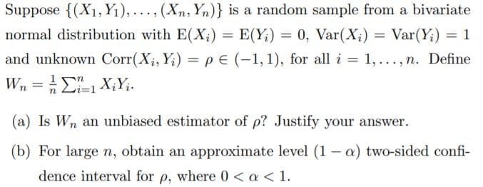
Suppose \(\left(X_{1}, Y_{1}\right), \ldots,\left(X_{n}, Y_{n}\right)\) is a random sample from a bivariate normal distribution with \(\mathrm{E}\left(X_{i}\right)=\mathrm{E}\left(Y_{i}\right)=0, Var\left(X_{i}\right)=Var\left(Y_{i}\right)=1\)
and unknown \(Corr\left(X_{i}, Y_{i}\right)=\rho \in(-1,1),\) for all \(i=1, \ldots, n .\) Define \(W_{n}=\frac{1}{n} \sum_{i=1}^{n} X_{i} Y_{i}\) a) Is \(W_{n}\) an unbiased estimator of \(\rho ?\) Justify your answer.
(b) For large \(n,\) obtain an approximate level \((1-\alpha)\) two-sided confi-
dence interval for \(\rho,\) where \(0<\alpha<1\).

Prerequisites

• Probability Theory (Expectation, Variance, Covariance, Correlation Coefficient)
• Unbiased Estimator
• Moments of Univariate Normal Distribution
• Bivariate Normal Distribution and a Different Definition
• Central Limit Theorem

Solution

(a)

Just compute the \(E(W_{n}\)).

\(E(W_{n})\) = \(\frac{1}{n} \sum_{i=1}^{n} E(X_{i} Y_{i})\) = \(\frac{1}{n} \sum_{i=1}^{n} \rho = \rho \).

\( \rho = E(X_{i} Y_{i}) - E(X_{i})E(Y_{i}) \overset{E(X_{i}) = E(Y_{i}) = 0}{=} E(X_{i} Y_{i})\).

So, \(W_{n}\) is unbiased for \( \rho \).

(b)

Observe that \(\left(X_{i}, Y_{i}\right)\) and \(\left(X_{j}, Y_{j}\right)\) are independent sample and therefore iid.

So, \(\left(X_{i}Y_{i}\right)\) and \(\left(X_{j}Y_{j}\right)\) are also iid.

Hence, computing the limiting distribution of \(W_{n}\), flashes in our minds, the Central Limit Theorem. So, let's dig into it. But, for that we need the following:

• \(E(W_{n}) = \rho \)
• \(Var(W_{n}) = \frac{1}{n} \sum_{i=1}^{n} Var(X_{i}Y_{i})\) = \(\frac{1}{n^2} \sum_{i=1}^{n} Var(X_{1}Y_{1}) = \frac{Var(X_{1}Y_{1})}{n} \overset{Why? Think}{=} \frac{E(({X_{1}Y_{1})^2)}}{n} \)

So, how to calculate the \({E((X_{1}Y_{1})^2)}\). For that

Two random variables \(X\) and \(Y\) are said to be jointly normal if they can be expressed in the form \(X = aU + bV, Y = cU + dV \), where \(U\) and \(V\) are independent standard normal random variables.

Alternate Definition of Bivariate Normal

Why do we need this? Because, \(X\) and \(Y\) are not independent and they have a correlation coefficient between them.

Assume, \((X, Y)\) ~ \((X_1, Y_1)\).

Exercise: Using the above result, prove that \(Y\) can be written as \( Y = \rho X + \sqrt{(1-\rho^2)}V\), where \(V\) ~ N(0,1) and \(V\) is independent of \(X\).

\(Y^2 = \rho^2X^2 + (1-\rho^2)V^2 + 2\rho\sqrt{(1-\rho^2)}XV\)

\(E(X^2Y^2) = E(\rho^2 X^4 + (1-\rho^2)X^2V^2 + 2\rho\sqrt{(1-\rho^2)}X^3V ) = \\ \rho^2E(X^4) + (1-\rho^2)E(X^2V^2) = \rho^2E(X^4) + (1-\rho^2)E(X^2)E(V^2) = 3\rho^2 + (1-\rho^2) = 1 + 2\rho^2\).

Exercise: Justify the above steps, using the independence of \(X\) and \(V\).

We used the fact that \(E(X^4) = 3\) if \(X\) ~ N(0,1). Instead of computing the whole we will use the fact that \( E(Z) = n\) and \(Var(Z) = 2n\) if \(Z\) ~ \( {{\chi}_n}^2\).

Exercise: Prove that \(E(X^4) = 3\) if \(X\) ~ N(0,1) using the above hint that \( X^2\) ~ \({{\chi}_1}^2\).

The final result, we got is the following:

\(Var(W_{n}) = \frac{1 + 2\rho^2}{n}\).
\(E(W_{n}) = \rho\).

Now use Central Limit Theorem.

\( \frac{\sqrt{n}(W_{n} - \rho)}{\sqrt{1 + 2\rho^2}} \to N(0, 1)\)

Therefore, \( P( |\frac{\sqrt{n}(W_{n} - \rho)}{\sqrt{1 + 2\rho^2}}| \leq z_{\alpha / 2} ) = (1-\alpha)\).

So, \( P(\left[W_{n} - z_{\alpha / 2} \left(\frac{\sqrt{1 + 2\rho^2}}{\sqrt{n}}\right) \leq \rho \leq W_{n} +z_{\alpha / 2} \left( \frac{\sqrt{1 + 2\rho^2}}{\sqrt{n}} \right) \right]) = (1-\alpha)\). Now, you have to square it to get a confidence interval for \(\rho^2\).

But, we can use variance stablizing transformation (pivotal method).

Observe that \(f(x) = \int \frac{1}{\sqrt{1+2u^2}} = ln|x+\sqrt{\frac{1}{2} + x^2} |\), which is an increasing and hence bijective function.

\( {\sqrt{n}(f(W_{n}) - f(\rho))} \to N(0, c)\). Calculate this constanc \( c = f'(\rho)^2.{\sqrt{1 + 2\rho^2}} \)

Now, try to find a confidence interval for \(f(\rho)\) based on this. Then take the inverse of \(f(x)\) to get a confidence interval for \(\rho\).

A Computational and Simulation Dimension

N <- 2000 # Number of random samples
# Target parameters for univariate normal distributions
v = NULL
rho <- 0.5
mu1 <- 0; s1 <- 1
mu2 <- 0; s2 <- 1
mu <- c(mu1,mu2) # Mean
sigma <- matrix(c(s1^2, s1*s2*rho, s1*s2*rho, s2^2),
                2) # Covariance matrix
library(MASS)
for (i in 1:1000) {
bvn1 <- mvrnorm(N, mu = mu, Sigma = sigma ) # from MASS package
W = bvn1[,1]*bvn1[,2]
Wbar = mean(W)
v = c(v, Wbar)
}
hist(v, freq =  F)
sigma2 = sqrt(1 + 2*rho^2)/sqrt(N)
x = seq(0.4, 0.6, 0.00001)
curve(dnorm(x, rho, sigma2), from = 0, col = "red", add = TRUE)

This problem was a bit more mathematical and technical, but still, I hope that the simulation along with the proofs gave you a good reading experience. Stay Tuned!