A simple convergence comparison between Leibniz's and mine pi formula

Author: Kazi Abu Rousan

Here there is $\pi$, there is circle.

Today's blog will be a bit different. This will not discuss any formula or any proof, rather it will just contain a python program to compare a $\pi$ formula given by Leibniz and a one discovered by me (blush).

How does Leibniz formula looks like?

The Leibniz formula for $\pi$ is named after Gottfried Leibniz( published in 1676). Sometimes it is also called Leibniz-Madhava series as this is actually a special case of a more general formula discovered by Madhava of Sangamagrama in 14th century.

The formula is:

$\frac{\pi}{4}$ = $1 - \frac{1}{3}$ + $\frac{1}{5}$ - $\frac{1}{7}$ + $\frac{1}{9}$ -$\cdots$ + $\frac{1}{4n+1}$ - $\frac{1}{4n+3}$ + $\cdots$

If you want a visual proof, read my article : Article- click

or this video: Geometric proof

So, how can you find $\pi$ using this?, Just calculate each fractions and add.

As an example, $4, 4(1-\frac{1}{3}) = 2.6667$, $4(1-\frac{1}{3}$ + $\frac{1}{5}) = 3.4664$, $4(1-\frac{1}{3}$ + $\frac{1}{5}$ - $\frac{1}{7}) =2.895238 $, just like this.

But it is nowhere close to the value of $\pi = 3.141592653\cdots$

The conclusion is that, it converges very slowly. Let's ask a computer to find the value of $\pi$ using the series.

pi_val = 3.1415926535897932#right value upto 17 decimals
calculated_pi_from_series = 0
n = 1000
for i in range(0,n):
    calculated_pi_from_series = calculated_pi_from_series + 1/(4*i+1) - 1/(4*i+3)
calculated_pi_from_series = 4*calculated_pi_from_series
print(calculated_pi_from_series)
print("error = ",pi_val - calculated_pi_from_series)
#output: 3.1410926536210413
#output: error =  0.0004999999687518297

For a output of $3.141592153589724$ and error $= 5.000000689037165e-07$, we need $n$ = $10,00,000$. As you can see slow this series is. But even then it has great mathematical significance. It even has a beautiful geometric relationship with Fermat's two square theorem and prime numbers.

How does my formula looks like?

As it is my own discovery, it doesn't have any name but you may call it Rousan's Formula (🤣🤣). This one is almost identical to Leibniz's formula. It is so as it also uses 2d complex numbers as it's basis just like Leibniz's formula.

The main difference is that it mine uses Eisenstein Integers, i.e., triangular grid while Leibniz's uses Gaussian Integers, i.e., regular square grid.

This formula can be written as :

$\frac{\pi}{3\sqrt{3}}$ = $1 - \frac{1}{2}$ + $\frac{1}{4}$ - $\frac{1}{5}$ + $\frac{1}{7}$ - $\cdots$ + $\frac{1}{3n+1}$ - $\frac{1}{3n+2}$ + $\cdots$

Almost same right?, now let's use python to see how fast it converges.

import math as mp
pi_val = 3.1415926535897932#right value upto 17 decimals
calculated_pi_from_series = 0
n = 1000
for i in range(0,n):
    calculated_pi_from_series = calculated_pi_from_series + 1/(3*i+1) - 1/(3*i+2)
calculated_pi_from_series = 3*calculated_pi_from_series*mp.sqrt(3)
print(calculated_pi_from_series)
print("error = ",pi_val - calculated_pi_from_series)
#output: 3.141015303363362
#output: error =  0.0005773502264312391

For $n = 10,00,000$, we get $3.1415920762392955$ with an error of $5.773504976325228e-07$. So, This shows mine converges a bit more slowly.

A direct comparison and reason

So, why mine converge more slowly?, well it is hidden in it's shape. Mine uses triangular grid and leibniz's uses squares. This is the main reason. But fear not, I have actually found a more generalized version of fermat's two square theorem, by using it i can get another similar series which converges faster than leibniz. Maybe I will discuss that in some later blog.

For now, let's try to plot both series's error. To we will plot the number of terms taken in x axis and error in y axis.

import matplotlib.pyplot as plt
import math as mp
pi_val = 3.1415926535897932
sqrt_3_3 = 3*mp.sqrt(3)

def leib_err(n):
    result = 0
    for i in range(n):
        result = result + 1/(4*i+1) - 1/(4*i+3)
    result = 4*result
    error = pi_val - result
    return result

def rou_err(n):
    result = 0
    for i in range(n):
        result = result + 1/(3*i+1) - 1/(3*i+2)
    result = result*sqrt_3_3
    error = pi_val - result
    return result
n_vals = [i for i in range(10_000+1)]
leibniz = [leib_err(i) for i in n_vals]
# print(leibniz)
rousan  =  [rou_err(i) for i in n_vals]
#
plt.plot(n_vals,leibniz,c='red',label='Leibniz Error')
plt.plot(n_vals,rousan,c='black',label='My formula Error')
plt.legend(loc='best',prop={'size':7})
plt.ylim(3.1375,3.1425)
plt.title("Error vs No. of terms for Leibniz and my $\\pi$ formula.")
plt.show()

The output is:

Error vs no. of terms for Leibniz and my pi formula
Error vs no. of terms for Leibniz and my pi formula - 2

This is all for today, see you guys next time with something new.

Your Personal Mandelbrot Set

Author: Kazi Abu Rousan

Bottomless wonders spring from simple rules, which are repeated without end.

Benoit Mandelbrot

Today, we will be discussing the idea for making a simple Mandelbrot Set using python's Matplotlib. This blog will not show you some crazy color scheme or such. But rather the most simple thing you can make from a simple code. So, Let's begin our discussion by understanding what is a Mandelbrot Set.

What is Mandelbrot Set?

In the most simple terms, The Mandelbrot set is the set of all complex numbers c for which the function $f_c(z) = z^2 + c$ doesn't goes to infinity when iterated from $z=0$.

Let's try to understand it using a example.

Suppose, we have a number $c = 1$, then to $ f_c(z)=f_1(z)= z^2 + 1 $.

Then, we first take $z_1 = f_1(z=0)=1$, after this we again calculate $z_2 = f_1(f_1(0)) = 1^2 + 1 = 2$, and so on. This goes on, i.e, we are getting new z values from the old one using $z_{n+1} = {z_n }^2 + 1$. This generates the series $0,1,2,5,26,\cdots$. As you can see, each element of this series goes to infinity, so the number $1$ is not an element of mandelbrot set.

Similarly, if we take $c=-1$, then the series is $0,-1,0.-1,0,\cdots$. This is a oscillating series and hence it will never grow towards infinity. Hence, the number $-1$ is an element of this set.

I hope this idea is now clear. It should be clear that $c$ can be any imaginary number. There is no restriction that says that $c$ must be real. So, is the number $c=i$ inside the set? Try it!!

Check if a Number is inside Mandelbrot set or not

Let's take a point $c = x+iy = P(x,y)$. So, the first point is $z_0 = 0+i\cdot 0 \to x = 0$ and $y=0$, i.e., we start the iteration from $f_c{z=0}$. Now, if at some point of iteration $|z_n|\geq 2$, then the corresponding $c$ value will not be inside the set. But if $|z|<2$, then corresponding c is inside the set.

Try this idea by hand for new numbers.

Now, let's check few numbers using a simple python code.

import numpy as np
def in_mandel(c,max_ita=1000):
    z = 0
    for i in range(max_ita):
        z = z**2 + c
        if abs(z)>=2:
            print(c," is not inside mandelbrot set upto a check of ",(i+1))
            break
        if i==max_ita-1 and abs(z)<2:
            print(c," is inside mandelbrot set upto a check of ",max_ita)
c1 = 1
in_mandel(c1)
#Output = 1  is not inside mandelbrot set
c2 = -1
in_mandel(c2)
#Output = -1  is inside mandelbrot set upto a check of  1000
c3 = 0.5+0.4j
in_mandel(c3)
#output = (0.5+0.4j)  is not inside mandelbrot set

You see how easy the code is!!, you can try out this geogebra version of you want - Check it here: Geogebra

Plot Mandelbrot set

Now, Let's plot one. We will be using a simple rule.

  1. If any number c is inside the set, we will mark that coordinate in the graph.
  2. If it is not there, we will just leave it.
import matplotlib.pyplot as plt
import numpy as np
max_ita = 1000 # number of interations
div = 1000 # divisions
c = np.linspace(-2,2,div)[:,np.newaxis] + 1j*np.linspace(-2,2,div)[np.newaxis,:]
z = 0 
for n in range(0,max_ita):
      z = z**2 + c
p = c[abs(z) < 2]#omit z which diverge 
plt.scatter(p.real, p.imag, color = "black" )
plt.xlabel("Real")
plt.grid(color='purple',linestyle='--')
plt.ylabel("i (imaginary)")
plt.xlim(-2,2)
plt.ylim(-1.5,1.5)
plt.show()

The output is:

Mandelbrot set
Mandelbrot set

This is not as good as the plots you normally see in internet like the images given below. But this one serves the purpose to show the shape of the set.

Let's try to make a bit fancier one.

The code is given here:

import matplotlib.pyplot as plt
import numpy as np
max_ita = 1000
div = 1000
c = np.linspace(-2,2,div)[:,np.newaxis] + 1j*np.linspace(-2,2,div)[np.newaxis,:] 
ones = np.ones(np.shape(c), np.int)
color = ones * max_ita + 5
z = 0
for n in range(0,max_ita):
      z = z**2 + c
      diverged = np.abs(z)>2
      color[diverged] = np.minimum(color[diverged], ones[diverged]*n)
plt.contourf(c.real, c.imag, color)
plt.xlabel("Real($c$)")
plt.ylabel("Imag($c$)")
plt.xlim(-2,2)
plt.ylim(-1.5,1.5)
plt.show()

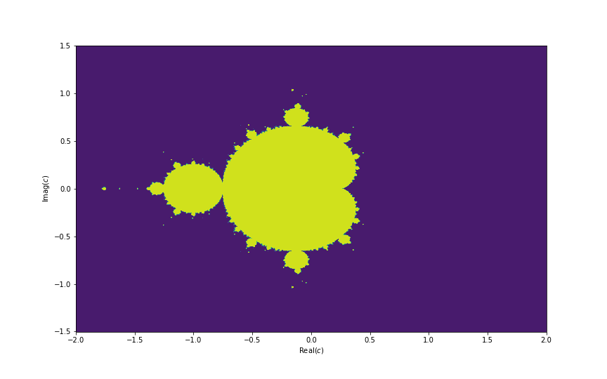
Here is the output:

Beautiful isn't it?, This set has many mystery. Like you can find the value of $\pi$ and Fibonacci number from it. It is also hidden in Bifurcation diagram and hence related to chaos theory.

But we will live all these mysteries for some later time. This is all for today. I hope you have enjoyed this and if you have, then don't forget to share.

Collatz Conjecture and a simple program

Author: Kazi Abu Rousan

Mathematics is not yet ready for such problems.

Paul Erdos

Introduction

A problem in maths which is too tempting and seems very easy but is actually a hidden demon is this Collatz Conjecture. This problems seems so easy that it you will be tempted, but remember it is infamous for eating up your time without giving you anything. This problem is so hard that most mathematicians doesn't want to even try it, but to our surprise it is actually very easy to understand. In this article our main goal is to understand the scheme of this conjecture and how can we write a code to apply this algorithm to any number again and again.

Note: If you are curious, the featured image is actually a visual representation of this collatz conjecture \ $3n+1$ conjecture. You can find the code here.

Statement and Some Examples

The statement of this conjecture can be given like this:

Suppose, we have any random positive integer $n$, we now use two operations:

Mathematically, we can write it like this:

$f(n) = \frac{n}{2}$ if $n \equiv 0$ (mod 2)

$ f(n) = (3n+1) $ if $n \equiv 1$ (mod 2)

Now, this conjecture says that no-matter what value of n you choose, you will always get 1 at the end of this operation if you perform it again and again.

Let's take an example, suppose we take $n=12$. As $12$ is an even number, we divide it by $2$. $\frac{12}{2} = 6$, which is again even. So, we again divide it by $2$. This time we get, $\frac{6}{2} = 3$, which is odd, hence, we multiply it by 3 and add $1$, i.e., $3\times 3 + 1 = 10$, which is again even. Hence, repeating this process we get the series $5 \to 16 \to 8 \to 4 \to 2 \to 1$. Seems easy right?,

Let's take again, another number $n=19$. This one gives us $19 \to 58 \to 29 \to 88 \to 44 \to 22 \to 11 \to 34 \to 17 \to 52 \to 26 \to 13 \to 40 \to 20 \to 10 \to 5 \to 16 \to 8 \to 4 \to 2 \to 1$. Again at the end we get $1$.

This time, we get much bigger numbers. There is a nice trick to visualize the high values, the plot which we use to do this is called Hailstone Plot.

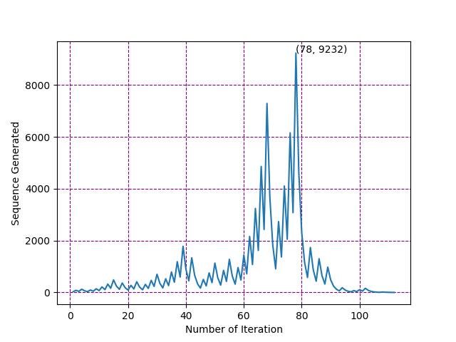
Let's take the number $n=27$. For this number, the list is $27 \to 82 \to 41 \to 124 \to 62 \to 31 \to 94 \to 47 \cdots \to 9232 \cdots$. As you can see, for this number it goes almost as high as 9232 but again it falls down to $1$. The hailstone plot for this is given below.

Hailstone for 27. The highest number and with it's iteration number is marked

So, what do you think is the conjecture holds for all number? , no one actually knows. Although, using powerful computers, we have verified this upto $2^{68}$. So, if you are looking for a counterexample, start from 300 quintillion!!

Generating the series for Collatz Conjecture for any number n using python

Let's start with coding part. We will be using numpy library.

import numpy as np
def collatz(n):
	result = np.array([n])
	while n >1:
		# print(n)
		if n%2 == 0:
			n = n/2
		else:
			n = 3*n + 1
		result = np.append(result,n)
	return result

The function above takes any number $n$ as it's argument. Then, it makes an array (think it as a box of numbers). It creates a box and then put $n$ inside it.

  1. Then for $n>1$, it check if $n$ is even or not.
  2. After this, if it is even then $n$ is divided by 2 and the previous value of n is replaced by $\frac{n}{2}$.
  3. And if $n$ is odd, the it's value is replaced by $3n+1$.
  4. For each case, we add the value of new $n$ inside our box of number. This whole process run until we have the value of $n=1$.
  5. Finally, we have the box of all number / series of all number inside the array result.

Let's see the result for $n = 12$.

n = 12
print(collatz(n))
#The output is: [12.  6.  3. 10.  5. 16.  8.  4.  2.  1.]

Similarly, for $n = 19$, the code gives us,

n = 19
print(collatz(n))
#The output is: [19. 58. 29. 88. 44. 22. 11. 34. 17. 52. 26. 13. 40. 20. 10.  5. 16.  8.  4.  2.  1.]

You can try out the code, it will give you the result for any number $n$.

Test this function.

Hailstone Plot

Now let's see how to plot Hailstone plot. Suppose, we have $n = 12$. In the image below, I have shown the series we get from $12$ using the algorithm.

Series and Step for $n=12$.

Now, as shown in the above image, we can assign natural numbers on each one of them as shown. So, Now we have two arraies (boxes), one with the series of numbers generated from $n$ and other one from the step number of the applied algorithm, i.e., series of natural numbers. Now, we can take elements from each series one by one and can generate pairs, i.e., two dimensional coordinates.

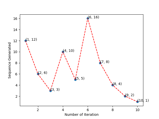
As shown in the above image, we can generate the coordinates using the steps as x coordinate and series a y coordinate. Now, if we plot the points, then that will give me Hailstone plot. For $n = 12$, we will get something like the image given below. Here I have simply added each dots with a red line.

The code to generate it is quite easy. We will be using matplotlib. We will just simply plot it and will mark the highest value along with it's corresponding step.

import numpy as np
import matplotlib.pyplot as plt
def collatz(n):
    result = np.array([n])
	while n >1:
		# print(n)
		if n%2 == 0:
			n = n/2
		else:
			n = 3*n + 1
		result = np.append(result,n)
	return result
n = 63728127
y_vals = collatz(n); x_vals = np.arange(1,len(y_vals)+1)
plt.plot(x_vals,y_vals)
x_val_max = np.where(y_vals == max(y_vals))[0][0]+1
plt.text(x_val_max, max(y_vals), '({}, {})'.format(x_val_max, int(max(y_vals))))
plt.grid(color='purple',linestyle='--')
plt.ylabel("Sequence Generated")
plt.xlabel("Number of Iteration")
plt.show()

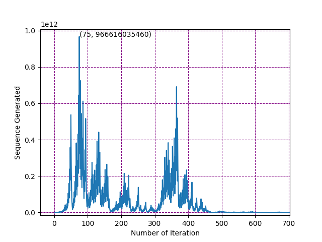
The output image is given below.

Crazy right?, you can try it out. It's almost feels like some sort of physics thing right!, for some it seems like stock market.

This is all for today. In it's part-2, we will go into much more detail. I hope you have learn something new.

Maybe in the part-2, we will see how to create pattern similar to this using collatz conjecture.

How to roll a Dice by tossing a Coin ? Cheenta Statistics Department

How can you roll a dice by tossing a coin? Can you use your probability knowledge? Use your conditioning skills.

Suppose, you have gone to a picnic with your friends. You have planned to play the physical version of the Snake and Ladder game. You found out that you have lost your dice.

The shit just became real!

Now, you have an unbiased coin in your wallet / purse. You know Probability.

Aapna Time Aayega

starts playing in the background. :p

Can you simulate the dice from the coin?

Ofcourse, you know chances better than others. :3

Take a coin.

Toss it 3 times. Record the outcomes.

HHH = Number 1

HHT = Number 2

HTH = Number 3

HTT = Number 4

THH = Number 5

THT = Number 6

TTH = Reject it, don't ccount the toss and toss again

TTT = Reject it, don't ccount the toss and toss again

Voila done!

What is the probability of HHH in this experiment?

Let X be the outcome in the restricted experiment as shown.

How is this experiment is different from the actual experiment?

This experiment is conditioning on the event A = {HHH, HHT, HTH, HTT, THH, THT}.

\(P( X = HHH) = P (X = HHH | X \in A ) = \frac{P (X = HHH)}{P (X \in A)} = \frac{1}{6}\)


Beautiful right?

Can you generalize this idea?

Food for thought

Watch the Video here:

Some Useful Links:

Books for ISI MStat Entrance Exam

How to Prepare for ISI MStat Entrance Exam

ISI MStat and IIT JAM Stat Problems and Solutions

Cheenta Statistics Program for ISI MStat and IIT JAM Stat

Simple Linear Regression - Playlist on YouTube

Circumference of a Semicircle | AMC 8, 2014 | Problem 25

Try this beautiful problem from AMC-8-2014 (Geometry) based on Circumference of a Semicircle

Circumference of a Semicircle- AMC 8, 2014 - Problem 25


On A straight one-mile stretch of highway, 40 feet wide, is closed. Robert rides his bike on a path composed of semicircles as shown. If he rides at 5miles per hour, how many hours will it take to cover the one-mile stretch?

circumference of a semicircle

  • \(\frac{\pi}{11}\)
  • \(\frac{\pi}{10}\)
  • \(\frac{\pi}{5}\)

Key Concepts


Geometry

Semicircle

Distance

Check the Answer


Answer:\(\frac{\pi}{10}\)

AMC-8, 2014 problem 25

Challenges and Thrills of Pre College Mathematics

Try with Hints


Find the circumference of a semi-circle

Can you now finish the problem ..........

If Robert rides in a straight line, it will take him \(\frac {1}{5}\) hours

can you finish the problem........

circumference of a semicircle

If Robert rides in a straight line, it will take him \(\frac {1}{5}\) hours. When riding in semicircles, let the radius of the semicircle r, then the circumference of a semicircle is \({\pi r}\). The ratio of the circumference of the semicircle to its diameter is \(\frac {\pi}{2}\). so the time Robert takes is  \(\frac{1}{5} \times \frac{\pi}{2}\). which is equal to \(\frac{\pi}{10}\)

Subscribe to Cheenta at Youtube


Spiral Similarity

Geometric Transformation is a powerful tool in Geometry. We look at one such transformation: Spiral Similarity.

Watch video

Try these Spiral Similarity problems. Send answers to helpdesk@cheenta.com

Problem 1: Suppose O = (0, 0), A = (2, 0) and B = (0, 2). Let T be the spiral similarity that sends A to B (center of T is O). What is the angle of spiral similarity? What is the dilation coefficient?

Problem 2: Can you rigorously prove the claim made at the end of the video?

Problem 3: Revisit the spiral similarity T described in problem 1. This can be realized by multiplying a complex number to A. What is that complex number?

Also try the problems related to Cyclic Quadrilaterals.

You may also click the link to learn its application:- https://www.youtube.com/watch?v=8o8AAWt960o

Using auxiliary polynomials in ISI Entrance

Auxiliary polynomials are useful for solving complicated polynomial problems. This problem from ISI Entrance (and a Soviet Olympiad) is a good example.

Watch video

Really understanding Direct Limit, Inverse Limit, and Hom

Direct Limit, Inverse Limit, and Hom are three ideas from category theory that are useful in many branches of mathematics. A deep understanding of them can be very helpful in the long run.

In the following video, we draw schematic pictures and gain real intuition behind these abstract ideas. This is clearly one of the most important videos of our production.

What is Inversive Geometry?

Inversion is one of several geometric transformations. It has a curious power of converting lines into circles. Inversion can be used to solve many geometry problems. It also has deep relations with complex numbers.

Watch the following video sequence to learn more about it.

The next video is coming up soon.

What if Fibonacci had a Torus?

Fibonacci Number matrix is closely related to Fibonacci numbers (no wonder)! They have a curious power to create curves on a torus. Welcome to the adventure!

Watch the first video

The next video will be live here shortly...