Lattice points on a circle - No. of solution of x^2+y^2 = N
Author: Kazi Abu Rousan
There are some problems in number theory which are very important not only because they came in exams but also they hide much richer intuition inside them. Today, we will be seeing one of such problems.
Sources:
B.Stat. (Hons.) and B.Math. (Hons.) I.S.I Admission Test 2012 problem-2.
B.Stat. (Hons.) and B.Math. (Hons.) I.S.I Admission Test 2015 problem-12.
The classical Gauss circle problem.
Problem:
The basic structure of the problem we are discussing is:
Find the number of solution of the equation $x^2+y^2 = N$ where $N \in \mathbb{N}$.
So, How to solve problems like this?, Here I will give you a formula to exactly find the number of solution for any general integer $N$.
Solution
The main idea behind these kind of problem is to use Fermat's Two-Square Theorem. So, what does the theorem says?
It says:
If any prime number $N$ is of the form $4k+1$, then $N$ can be written as $x^2+y^2$ for some $x,y \in \mathbb{I} $. This means if $N$ is of the form $4k+3$, then $x^2+y^2=N$ doesn't have any solution.
This gives us our answer if $N$ is a prime number. So, if the problem is to find the number of solution of $x^2+y^2 = 2003$ or maybe $3, 7, \cdots , 23, \cdots $, i.e., any prime with the remainder of $3$ when divided by 4, then we directly know that the number of solution is zero.
So, we have a method to solve these type of problems for prime $N$. But what about non-prime numbers?
For the case of non-prime numbers, I will just give you the formula and will show you how to use that. If you want to know how we got the formula or the details of the formula, you can just watch my lecture.
The formula to calculate the number of solution for $N = p_0^{a_0} p_1^{a_1} \cdots p_{n-1}^{a_{n-1}}$
$$\text{ No of soln } = 4\cdot \Pi_{i=0}^{n-1}\Big(\sum_{j=0}^{a_i} \chi(p_i ^{j}) \Big)$$
or in simple terms,
$$\text{ No of soln } = 4\cdot (\chi(p_0^0)+\chi(p_0^1)+\cdots + \chi(p_0^{a_0}))\cdot ( \chi(p_1^0)+\chi(p_1^1)+\cdots + \chi(p_1^{a_1}) ) \cdots $$
Where $\chi$ is a number theoretical function defined as,
So, the number of solutions is, $ n = 4\times (\chi(2^0)+\chi(2^1))\times (\chi(3^0)+\chi(3^1) + \chi(3^2)) \times (\chi(5^0)+\chi(5^1)+\chi(5^2)+\chi(5^3))$.
Now, from definition, $\chi(1) = 1$, $\chi(2) = 0$, $\chi(3) = -1$ and $\chi(5) = 1$. And also $\chi(x^n) = \chi(x)^n$, hence
If you are a person who loves to read maths related stuff then sure you have came across the words Riemann Zeta function and Riemann Hypothesis at least once. But today we are not going into the Riemann Hypothesis, rather we are going into the Zeta Function. To be more specific, we will see how to calculate the value of zeta function using a simple Julia Program only for $Re(input)>1$.
What is Zeta Function?
What is the Zeta Function?
The Riemann zeta function $\zeta (s)$ is a function of a complex variables $z = \sigma + i t $. When $Re(z) = \sigma >1$, we can define this as a converging summation given by,
There are many methods to calculate the values of this function for each value of $n$. You can surely do this by hand although I can't suggest that. The easiest way will be to utilize program.
Code to find the value of zeta for Re(z)>1
Before writing the code, you should remember that the sum is actually infinite. Hence, our function will give us more and more fine result as we include more and more terms.
function ζ(z,limit=1000)
    result = 0
    for i in 1:limit
        result += (1/i)^z
    end
    return result
end
This is the function. How simple!!.. and If we use julia as you can see, we can actually use $\zeta $ symbol. Pretty cool right?
ζ(2,10_0000_000)
#Output: 1.644934057834575
#where pi^2/6 = 1.6449340668482264
#pretty close
It's not all. We can actually apply this function to find the value of zeta function for complex inputs too.
When we use complex inputs, there is a beautiful hidden beauty. Let's see that using a plotting library called Plots and we also have to rewrite our function a little bit.
function ζ(z,limit=1000;point_ar = false)
    points = ComplexF64[0]
    result = 0
    for i in 1:limit
        result += (1/i)^z
        if point_ar
            push!(points,result)
        end
    end
    return result, points
end
Now, we can use this to plot.
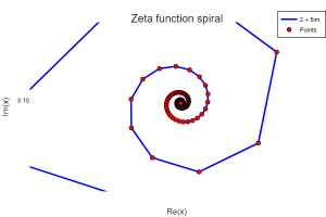
z = 2+5im
result, points = ζ(z;point_ar = true)
plot((points),color=:blue,width=3, title="Zeta function spiral",framestyle= :origin,label="$z")
scatter!((points),color=:red, label="Points")S
The output is:
The complex power rotates each point.Zoomed Image of the spiral
Who would have thought that there will be something like this hidden.
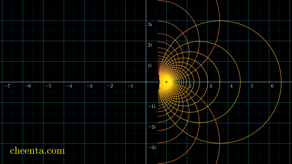
Now, If we apply this function to all possible points of the NumberPlane, then we will get a mesmerizing pattern.
Beautiful!!! But why is it feels like incomplete?
Looking at the image it feels like It's begging to be extended to the other portion. This extension is done using something we called Analytic Continuation. We will not go into much detail here.
If you want to know about the remaining story visit by lecture here:
This is all for today. Why not try to extend the idea to the other side?
Hope you learnt something new.
Your Personal Mandelbrot Set
Author: Kazi Abu Rousan
Bottomless wonders spring from simple rules, which are repeated without end.
Benoit Mandelbrot
Today, we will be discussing the idea for making a simple Mandelbrot Set using python's Matplotlib. This blog will not show you some crazy color scheme or such. But rather the most simple thing you can make from a simple code. So, Let's begin our discussion by understanding what is a Mandelbrot Set.
What is Mandelbrot Set?
In the most simple terms, The Mandelbrot set is the set of all complex numbers c for which the function $f_c(z) = z^2 + c$ doesn't goes to infinity when iterated from $z=0$.
Let's try to understand it using a example.
Suppose, we have a number $c = 1$, then to $ f_c(z)=f_1(z)= z^2 + 1 $.
Then, we first take $z_1 = f_1(z=0)=1$, after this we again calculate $z_2 = f_1(f_1(0)) = 1^2 + 1 = 2$, and so on. This goes on, i.e, we are getting new z values from the old one using $z_{n+1} = {z_n }^2 + 1$. This generates the series $0,1,2,5,26,\cdots$. As you can see, each element of this series goes to infinity, so the number $1$ is not an element of mandelbrot set.
Similarly, if we take $c=-1$, then the series is $0,-1,0.-1,0,\cdots$. This is a oscillating series and hence it will never grow towards infinity. Hence, the number $-1$ is an element of this set.
I hope this idea is now clear. It should be clear that $c$ can be any imaginary number. There is no restriction that says that $c$ must be real. So, is the number $c=i$ inside the set? Try it!!
Check if a Number is inside Mandelbrot set or not
Let's take a point $c = x+iy = P(x,y)$. So, the first point is $z_0 = 0+i\cdot 0 \to x = 0$ and $y=0$, i.e., we start the iteration from $f_c{z=0}$. Now, if at some point of iteration $|z_n|\geq 2$, then the corresponding $c$ value will not be inside the set. But if $|z|<2$, then corresponding c is inside the set.
Try this idea by hand for new numbers.
Now, let's check few numbers using a simple python code.
import numpy as np
def in_mandel(c,max_ita=1000):
    z = 0
    for i in range(max_ita):
        z = z**2 + c
        if abs(z)>=2:
            print(c," is not inside mandelbrot set upto a check of ",(i+1))
            break
        if i==max_ita-1 and abs(z)<2:
            print(c," is inside mandelbrot set upto a check of ",max_ita)
c1 = 1
in_mandel(c1)
#Output = 1  is not inside mandelbrot set
c2 = -1
in_mandel(c2)
#Output = -1  is inside mandelbrot set upto a check of  1000
c3 = 0.5+0.4j
in_mandel(c3)
#output = (0.5+0.4j)  is not inside mandelbrot set
You see how easy the code is!!, you can try out this geogebra version of you want - Check it here: Geogebra
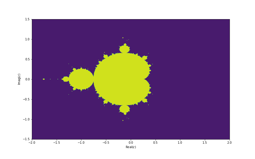
Plot Mandelbrot set
Now, Let's plot one. We will be using a simple rule.
If any number c is inside the set, we will mark that coordinate in the graph.
If it is not there, we will just leave it.
import matplotlib.pyplot as plt
import numpy as np
max_ita = 1000 # number of interations
div = 1000 # divisions
c = np.linspace(-2,2,div)[:,np.newaxis] + 1j*np.linspace(-2,2,div)[np.newaxis,:]
z = 0
for n in range(0,max_ita):
      z = z**2 + c
p = c[abs(z) < 2]#omit z which diverge
plt.scatter(p.real, p.imag, color = "black" )
plt.xlabel("Real")
plt.grid(color='purple',linestyle='--')
plt.ylabel("i (imaginary)")
plt.xlim(-2,2)
plt.ylim(-1.5,1.5)
plt.show()
The output is:
Mandelbrot set
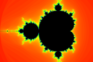
This is not as good as the plots you normally see in internet like the images given below. But this one serves the purpose to show the shape of the set.
Let's try to make a bit fancier one.
The code is given here:
import matplotlib.pyplot as plt
import numpy as np
max_ita = 1000
div = 1000
c = np.linspace(-2,2,div)[:,np.newaxis] + 1j*np.linspace(-2,2,div)[np.newaxis,:]
ones = np.ones(np.shape(c), np.int)
color = ones * max_ita + 5
z = 0
for n in range(0,max_ita):
      z = z**2 + c
      diverged = np.abs(z)>2
      color[diverged] = np.minimum(color[diverged], ones[diverged]*n)
plt.contourf(c.real, c.imag, color)
plt.xlabel("Real($c$)")
plt.ylabel("Imag($c$)")
plt.xlim(-2,2)
plt.ylim(-1.5,1.5)
plt.show()
Here is the output:
Beautiful isn't it?, This set has many mystery. Like you can find the value of $\pi$ and Fibonacci number from it. It is also hidden in Bifurcation diagram and hence related to chaos theory.
But we will live all these mysteries for some later time. This is all for today. I hope you have enjoyed this and if you have, then don't forget to share.
Collatz Conjecture and a simple program
Author: Kazi Abu Rousan
Mathematics is not yet ready for such problems.
Paul Erdos
Introduction
A problem in maths which is too tempting and seems very easy but is actually a hidden demon is this Collatz Conjecture. This problems seems so easy that it you will be tempted, but remember it is infamous for eating up your time without giving you anything. This problem is so hard that most mathematicians doesn't want to even try it, but to our surprise it is actually very easy to understand. In this article our main goal is to understand the scheme of this conjecture and how can we write a code to apply this algorithm to any number again and again.
Note: If you are curious, the featured image is actually a visual representation of this collatz conjecture \ $3n+1$ conjecture. You can find the code here.
Statement and Some Examples
The statement of this conjecture can be given like this:
Suppose, we have any random positive integer $n$, we now use two operations:
If the number n is even, divide it by $2$.
If the number is odd, triple it and add $1$.
Mathematically, we can write it like this:
$f(n) = \frac{n}{2}$ if $n \equiv 0$ (mod 2)
$ f(n) = (3n+1) $ if $n \equiv 1$ (mod 2)
Now, this conjecture says that no-matter what value of n you choose, you will always get 1 at the end of this operation if you perform it again and again.
Let's take an example, suppose we take $n=12$. As $12$ is an even number, we divide it by $2$. $\frac{12}{2} = 6$, which is again even. So, we again divide it by $2$. This time we get, $\frac{6}{2} = 3$, which is odd, hence, we multiply it by 3 and add $1$, i.e., $3\times 3 + 1 = 10$, which is again even. Hence, repeating this process we get the series $5 \to 16 \to 8 \to 4 \to 2 \to 1$. Seems easy right?,
Let's take again, another number $n=19$. This one gives us $19 \to 58 \to 29 \to 88 \to 44 \to 22 \to 11 \to 34 \to 17 \to 52 \to 26 \to 13 \to 40 \to 20 \to 10 \to 5 \to 16 \to 8 \to 4 \to 2 \to 1$. Again at the end we get $1$.
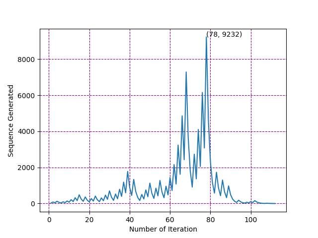
This time, we get much bigger numbers. There is a nice trick to visualize the high values, the plot which we use to do this is called Hailstone Plot.
Let's take the number $n=27$. For this number, the list is $27 \to 82 \to 41 \to 124 \to 62 \to 31 \to 94 \to 47 \cdots \to 9232 \cdots$. As you can see, for this number it goes almost as high as 9232 but again it falls down to $1$. The hailstone plot for this is given below.
Hailstone for 27. The highest number and with it's iteration number is marked
So, what do you think is the conjecture holds for all number? , no one actually knows. Although, using powerful computers, we have verified this upto $2^{68}$. So, if you are looking for a counterexample, start from 300 quintillion!!
Generating the series for Collatz Conjecture for any number n using python
Let's start with coding part. We will be using numpy library.
import numpy as np
def collatz(n):
	result = np.array([n])
	while n >1:
		# print(n)
		if n%2 == 0:
			n = n/2
		else:
			n = 3*n + 1
		result = np.append(result,n)
	return result
The function above takes any number $n$ as it's argument. Then, it makes an array (think it as a box of numbers). It creates a box and then put $n$ inside it.
Then for $n>1$, it check if $n$ is even or not.
After this, if it is even then $n$ is divided by 2 and the previous value of n is replaced by $\frac{n}{2}$.
And if $n$ is odd, the it's value is replaced by $3n+1$.
For each case, we add the value of new $n$ inside our box of number. This whole process run until we have the value of $n=1$.
Finally, we have the box of all number / series of all number inside the array result.
Let's see the result for $n = 12$.
n = 12
print(collatz(n))
#The output is: [12.  6.  3. 10.  5. 16.  8.  4.  2.  1.]
You can try out the code, it will give you the result for any number $n$.
Test this function.
Hailstone Plot
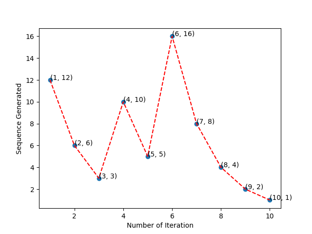
Now let's see how to plot Hailstone plot. Suppose, we have $n = 12$. In the image below, I have shown the series we get from $12$ using the algorithm.
Series and Step for $n=12$.
Now, as shown in the above image, we can assign natural numbers on each one of them as shown. So, Now we have two arraies (boxes), one with the series of numbers generated from $n$ and other one from the step number of the applied algorithm, i.e., series of natural numbers. Now, we can take elements from each series one by one and can generate pairs, i.e., two dimensional coordinates.
As shown in the above image, we can generate the coordinates using the steps as x coordinate and series a y coordinate. Now, if we plot the points, then that will give me Hailstone plot. For $n = 12$, we will get something like the image given below. Here I have simply added each dots with a red line.
The code to generate it is quite easy. We will be using matplotlib. We will just simply plot it and will mark the highest value along with it's corresponding step.
import numpy as np
import matplotlib.pyplot as plt
def collatz(n):
result = np.array([n])
while n >1:
# print(n)
if n%2 == 0:
n = n/2
else:
n = 3*n + 1
result = np.append(result,n)
return result
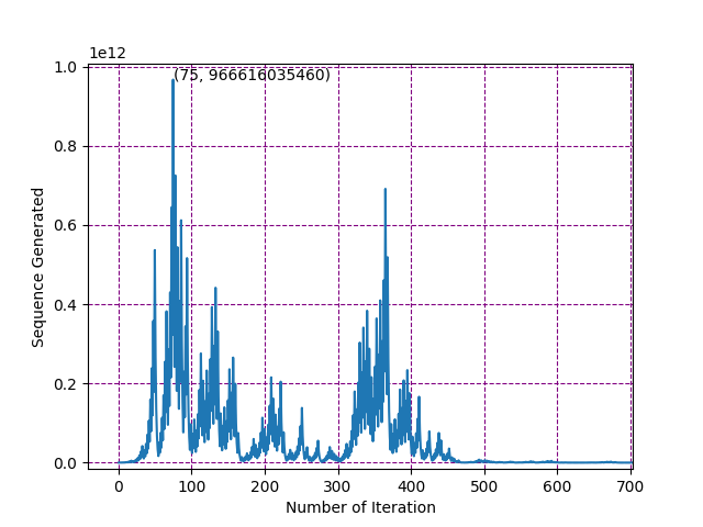
n = 63728127
y_vals = collatz(n); x_vals = np.arange(1,len(y_vals)+1)
plt.plot(x_vals,y_vals)
x_val_max = np.where(y_vals == max(y_vals))[0][0]+1
plt.text(x_val_max, max(y_vals), '({}, {})'.format(x_val_max, int(max(y_vals))))
plt.grid(color='purple',linestyle='--')
plt.ylabel("Sequence Generated")
plt.xlabel("Number of Iteration")
plt.show()
The output image is given below.
Crazy right?, you can try it out. It's almost feels like some sort of physics thing right!, for some it seems like stock market.
This is all for today. In it's part-2, we will go into much more detail. I hope you have learn something new.
Maybe in the part-2, we will see how to create pattern similar to this using collatz conjecture.
Gaussian Prime Spiral and Its beautiful Patterns
Author: Kazi Abu Rousan
Mathematics is the science of patterns, and nature exploits just about every pattern that there is.
Ian Stewart
Introduction
If you are a math enthusiastic, then you must have seen many mysterious patterns of Prime numbers. They are really great but today, we will explore beautiful patterns of a special type of 2-dimensional primes, called Gaussian Primes. We will focus on a very special pattern of these primes, called the Gaussian Prime Spiral. First, we have understood what those primes are. The main purpose of this article is to show you guys how to utilize programming to analyze beautiful patterns of mathematics. So, I have not given any proof, rather we will only focus on the visualization part.
Gaussian Integers and Primes
We all know about complex numbers right? They are the number of form $z=a+bi$, were $i$ = $\sqrt{-1}$. They simply represent points in our good old coordinate plane. Like $z=a+bi$ represent the point $(a,b)$. This means every point on a 2d graph paper can be represented by a Complex number.
In python, we write $i$ = $\sqrt{-1}$ as $1j$. So, we can write any complex number $z$ = $2 + 3i$ as $z$ = $2+1j*3$. As an example, see the piece of code below.
z = 2 + 1j*3print(z)
#output is (2+3j)
print(type(z))
#output is <class 'complex'>
#To verify that it indeed gives us complex number, we can see it by product law.
z1 = 2 + 1j*3z2 = 5 + 1j*2print(z1*z2)
#output is (4+19j)
To access the real and imaginary components individually, we use the real and imag command. Hence, z.real will give us 2 and z.imag will give us 3. We can use abs command to find the absolute value of any complex number, i.e., abs(z) = $\sqrt{a^2+b^2} = \sqrt{2^2+1^2}= \sqrt{5}$. Here is the example code.
print(z.real)
#Output is 2.0
print(z.imag)
#output is 3.0
print(abs(z))
#Output is 3.605551275463989
If lattice points, i.e., points with integer coordinates (eg, (2,3), (6,13),... etc) on the coordinate plane (like the graph paper you use in your class) are represented as complex numbers, then they are called Gaussian Integers. Like we can write (2,3) as $2+3i$. So, $2+3i$ is a Gaussian Integer.
Gaussian Primes are almost same in $\mathbb{Z}[i]$ as ordinary primes are in $\mathbb{Z_{+}}$, i.e., Gaussian Primes are complex numbers that cannot be further factorized in the field of complex numbers. As an example, $5+3i$ can be factorised as $(1+i)(3-2i)$. So, It is not a gaussian prime. But $3-2i$ is a Gaussian prime as it cannot be further factorized. Likewise, 5 can be factorised as $(2+i)(2-i)$. So it is not a gaussian prime. But we cannot factorize 3. Hence, $3+0i$ is a gaussian prime.
Note: Like, 1 is not a prime in the field of positive Integers, $i$ and also $1$ are not gaussian prime in the field of complex numbers. Also, you can define what a Gaussian Prime is, using the 2 condition given below (which we have used to check if any $a+ib$ is a gaussian prime or not).
Checking if a number is Gaussian prime or not
Now, the question is, How can you check if any given Gaussian Integer is prime or not? Well, you can use try and error. But it's not that great. So, to find if a complex number is gaussian prime or not, we will take the help of Fermat's two-square theorem.
A complex number $z = a + bi$ is a Gaussian prime, if:. As an example, $5+0i$ is not a gaussian prime as although its imaginary component is zero, its real component is not of the form $4n+3$. But $3i$ is a Gaussian prime, as its real component is zero but the imaginary component, 3 is a prime of the form $4n+3$.
One of $|a|$ or $|b|$ is zero and the other one is a prime number of form $4n+3$ for some integer $n\geq 0$. As an example, $5+0i$ is a gaussian prime as although it's imaginary component is zero, it's real component is not of the form $4n+3$. But $3i$ is a gaussian prime, as it's real component is zero and imaginary component, 3 is a prime of form $4n+3$.
If both a and b are non-zero and $(abs(z))^2=a^2+b^2$ is a prime. This prime will be of the form $4n+1$.
Using this simple idea, we can write a python code to check if any given Gaussian integer is Gaussian prime or not. But before that, I should mention that we are going to use 2 libraries of python:
matplotlib $\to$ This one helps us to plot different plots to visualize data. We will use one of it's subpackage (pyplot).
sympy $\to$ This will help us to find if any number is prime or not. You can actually define that yourself too. But here we are interested in gaussian primes, so we will take the function to check prime as granted.
So, the function to check if any number is gaussian prime or not is,
import numpy as np
import matplotlib.pyplot as plt
from sympy import isprimedef gprime(z):#check if z is gaussian prime or not, return true or false
re = int(abs(z.real)); im = int(abs(z.imag))
if re == 0 and im == 0:
return False
d = (re**2+im**2)
if re != 0 and im != 0:
return isprime(d)
if re == 0 or im == 0:
abs_val = int(abs(z))
if abs_val % 4 == 3:
return isprime(abs_val)
else:
return False
Let's test this function.
print(gprime(1j*3))
#output is True
print(gprime(5))
#output is False
print(gprime(4+1j*5))
#output is True
Let's now plot all the Gaussian primes within a radius of 100. There are many ways to do this, we can first define a function that returns a list containing all Gaussian primes within the radius n, i.e., Gaussian primes, whose absolute value is less than or equals to n. The code can be written like this (exercise: Try to increase the efficiency).
def gaussian_prime_inrange(n):
    gauss_pri = []
    for a in range(-n,n+1):
        for b in range(-n,n+1):
            gaussian_int = a + 1j*b
            if gprime(gaussian_int):
                gauss_pri.append(gaussian_int)
    return gauss_pri
Now, we can create a list containing all Gaussian primes in the range of 100.
To plot all these points, we need to separate the real and imaginary parts. This can be done using the following code.
gaussian_p_real = [x.real for x in gaussain_pri_array]
gaussian_p_imag = [x.imag for x in gaussain_pri_array]
The code to plot this is here (exercise: Play around with parameters to generate a beautiful plot).
plt.axhline(0,color='Black');plt.axvline(0,color='Black') # Draw re and im axis
plt.scatter(gaussian_p_real,gaussian_p_imag,color='red',s=0.4)
plt.xlabel("Re(z)")
plt.ylabel("Im(z)")
plt.title("Gaussian Primes")
plt.savefig("gauss_prime.png", bbox_inches = 'tight',dpi = 300)
plt.show()
Look closely, you can find a pattern... maybe try plotting some more primes
Gaussian Prime Spiral
Now, we are ready to plot the Gaussian prime spiral. I have come across these spirals while reading the book Learning Scientific Programming with Python, 2nd edition, written by Christian Hill. There is a particular problem, which is:
Although, history is far richer than just solving a simple problem. If you are interested try this article: Stepping to Infinity Along Gaussian Primes by Po-Ru Loh (The American Mathematical Monthly, vol-114, No. 2, Feb 2007, pp. 142-151). But here, we will just focus on the problem. Maybe in the future, I will explain this article in some video.
The plot of the path will be like this:
Beautiful!! Isn't it? Before seeing the code, let's try to understand how to draw this by hand. Let's take the initial point as $c_0=3+2i$ and $\Delta c = 1+0i=1$.
For the first step, we don't care if $c_0$ is gaussian prime or not. We just add the step with it, i.e., we add $\Delta c$ with $c_0$. For our case it will give us $c_1=(3+2i)+1=4+2i$.
Then, we check if $c_1$ is a gaussian prime or not. In our case, $c_1=4+2i$ is not a gaussian prime. So, we repeat step-1(i.e., add $\Delta c$ with it). This gives us $c_2=5+2i$. Again we check if $c_2$ is gaussian prime or not. In this case, $c_2$ is a gaussian prime. So, now we have to rotate the direction $90^{\circ}$ towards the left,i.e., anti-clockwise. In complex plane, it is very easy. Just multiply the $\Delta c$ by $i = \sqrt{-1}$ and that will be our new $\Delta c$. For our example, $c_3$ = $c_2+\Delta c$ = $5+2i+(1+0i)\cdot i$ = $5+3i$.
From here, again we follow step-2, until we get the point from where we started with the same $\Delta c$ or you can do it for your required step.
The list of all the complex number we will get for this particular example is:
Index
Complex No.
Step
Index
Complex No.
Step
0
$3+2i$
+1
7
$2+4i$
-1
1
$4+2i$
+1
8
$1+4i$
-i
2
$5+2i$
+i
9
$1+3i$
-i
3
$5+3i$
+i
10
$1+2i$
+1
4
$5+4i$
-1
11
$2+2i$
+1
5
$4+4i$
-1
12
$3+2i$
+i
6
$3+4i$
-1
13
$3+3i$
+i
Complex numbers and $\Delta c$'s along Gaussian prime spiral
Note that although $c_{12}$ is the same as $c_0$, as it is a Gaussian prime, the next gaussian integer will be different from $c_1$. This is the case because $\Delta c$ will be different.
To plot this, just take each $c_i$ as coordinate points, and add 2 consecutive points with a line. The path created by the lines is called a Gaussian prime spiral. Here is a hand-drawn plot.
I hope now it is clear how to plot this type of spiral. You can use the same concept for Eisenstein primes, which are also a type of 2D primes to get beautiful patterns (Excercise: Try these out for Eisenstein primes, it will be a little tricky).
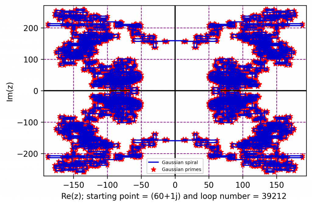
We can define our function to find points of the gaussian prime spiral such that it only contains as many numbers as we want. Using that, let's plot the spiral for $c_0 = 3+2i$, which only contains 30 steps.
Here is the code to generate it. Try to analyze it.
def gaussian_spiral(seed, loop_num = 1, del_c = 1, initial_con = True):#Initial condition is actually the fact
#that represnet if you want to get back to the initial number(seed) at the end.
    d = seed; gaussian_primes_y = []; gaussian_primes_x = []
    points_x = [d.real]; points_y = [d.imag]
    if initial_con:
        while True:
            seed += del_c; real = seed.real; imagi = seed.imag
            points_x.append(real); points_y.append(imagi)
            if seed == d:
                break
            if gprime(seed):
                del_c *= 1j
                gaussian_primes_x.append(real); gaussian_primes_y.append(imagi)
    else:
        for i in range(loop_num):
            seed += del_c; real = seed.real; imagi = seed.imag
            points_x.append(real); points_y.append(imagi)
            if gprime(seed):
                del_c *= 1j ;
                gaussian_primes_x.append(real); gaussian_primes_y.append(imagi)
    gauss_p = [gaussian_primes_x,gaussian_primes_y]
    return points_x, points_y, gauss_p
Using this piece of code, we can literally generate any gaussian prime spiral. Like, for the problem of the book, here is the solution code:
Also, you can use python using an android app - Pydroid 3 (which is free)
I have also written this in Julia. Julia is faster than Python. Here you can find Julia's version: https://zurl.co/wETi
Amplitude and Complex numbers | AIME I, 1996 Question 11
Try this beautiful problem from the American Invitational Mathematics Examination I, AIME I, 1996 based on Amplitude and Complex numbers.
Amplitude and Complex numbers - AIME 1996
Let P be the product of the roots of \(z^{6}+z^{4}+z^{2}+1=0\) that have a positive imaginary part and suppose that P=r(costheta+isintheta) where \(0 \lt r\) and \(0 \leq \theta \lt 360\) find \(\theta\)
is 107
is 276
is 840
cannot be determined from the given information
Key Concepts
Equations
Complex Numbers
Integers
Check the Answer
Answer: is 276.
AIME, 1996, Question 11
Complex Numbers from A to Z by Titu Andreescue
Try with Hints
here\(z^{6}+z^{4}+z^{2}+1\)=\(z^{6}-z+z^{4}+z^{2}+z+1\)=\(z(z^{5}-1)+\frac{(z^{5}-1)}{(z-1)}\)=\(\frac{(z^{5}-1)(z^{2}-z+1)}{(z-1)}\) then \(\frac{(z^{5}-1)(z^{2}-z+1)}{(z-1)}\)=0
gives \(z^{5}=1 for z\neq 1\) gives \(z=cis 72,144,216,288\) and \(z^{2}-z+1=0 for z \neq 1\) gives z=\(\frac{1+-(-3)^\frac{1}{2}}{2}\)=\(cis60,300\) where cis\(\theta\)=cos\(\theta\)+isin\(\theta\)
taking \(0 \lt theta \lt 180\) for positive imaginary roots gives cis72,60,144 and then P=cis(72+60+144)=cis276 that is theta=276.
This is a beautiful problem from ISI MSTAT 2015 PSA problem 18 based on complex number. We provide sequential hints so that you can try.
Complex Number - ISI MStat Year 2015 PSA Question 18
The set of complex numbers $z$ satisfying the equation \( (3+7 i) z+(10-2 i) \bar{z}+100=0\) represents, in the complex plane
a straight line
a pair of intersecting straight lines
a point
a pair of distinct parallel straight lines
Key Concepts
Complex number representation
Straight line
Check the Answer
Answer: is a pair of intersecting straight lines
ISI MStat 2015 PSA Problem 18
Precollege Mathematics
Try with Hints
Simplify the Complex. Just Solve.
Let \(z = x+iy, \bar{z} = x-iy\) Then the given equation reduces to \((13x-9y+100)+i(5x-7y) = 0\). Which implies \(13x-9y+100 = 0, 5x-7y = 0\). They do intersect.(?)
Yes! they intersect and to get the point of intersection just use substitution . Hence it gives a pair of intersecting straight lines.
Problem on Complex plane | AIME I, 1988| Question 11
Try this beautiful problem from the American Invitational Mathematics Examination I, AIME I, 1988 based on Complex Plane.
Problem on Complex Plane - AIME I, 1988
Let w_1,w_2,....,w_n be complex numbers. A line L in the complex plane is called a mean line for the points w_1,w_2,....w_n if L contains points (complex numbers) z_1,z_2, .....z_n such that \(\sum_{k=1}^{n}(z_{k}-w_{k})=0\) for the numbers \(w_1=32+170i, w_2=-7+64i, w_3=-9+200i, w_4=1+27i\) and \(w_5=-14+43i\), there is a unique mean line with y-intercept 3. Find the slope of this mean line.
is 107
is 163
is 634
cannot be determined from the given information
Key Concepts
Integers
Equations
Algebra
Check the Answer
Answer: is 163.
AIME I, 1988, Question 11
Elementary Algebra by Hall and Knight
Try with Hints
\(\sum_{k=1}^{5}w_k=3+504i\)
and \(\sum_{k-1}^{5}z_k=3+504i\)
taking the numbers in the form a+bi
\(\sum_{k=1}^{5}a_k=3\) and \(\sum_{k=1}^{5}b_k=504\)
or, y=mx+3 where \(b_k=ma_k+3\) adding all 5 equations given for each k
Complex numbers and Sets | AIME I, 1990 | Question 10
Try this beautiful problem from the American Invitational Mathematics Examination I, AIME I, 1990 based on Complex Numbers and Sets.
Complex Numbers and Sets - AIME I, 1990
The sets A={z:\(z^{18}=1\)} and B={w:\(w^{48}=1\)} are both sets of complex roots with unity, the set C={zw: \(z \in A and w \in B\)} is also a set of complex roots of unity. How many distinct elements are in C?.
is 107
is 144
is 840
cannot be determined from the given information
Key Concepts
Integers
Complex Numbers
Sets
Check the Answer
Answer: is 144.
AIME I, 1990, Question 10
Complex Numbers from A to Z by Titu Andreescue
Try with Hints
18th and 48th roots of 1 found by de Moivre's Theorem
=\(cis(\frac{2k_1\pi}{18})\) and \(cis(\frac{2k_2\pi}{48})\)
where \(k_1\), \(K_2\) are integers from 0 to 17 and 0 to 47 and \(cis \theta = cos \theta +i sin \theta\)
Complex roots and equations | AIME I, 1994 | Question 13
Try this beautiful problem from the American Invitational Mathematics Examination I, AIME I, 1995 based on Complex roots and equations.
Complex roots and equations - AIME I, 1994
\(x^{10}+(13x-1)^{10}=0\) has 10 complex roots \(r_1\), \(\overline{r_1}\), \(r_2\),\(\overline{r_2}\).\(r_3\),\(\overline{r_3}\),\(r_4\),\(\overline{r_4}\),\(r_5\),\(\overline{r_5}\) where complex conjugates are taken, find the values of \(\frac{1}{(r_1)(\overline{r_1})}+\frac{1}{(r_2)(\overline{r_2})}+\frac{1}{(r_3)(\overline{r_3})}+\frac{1}{(r_4)(\overline{r_4})}+\frac{1}{(r_5)(\overline{r_5})}\)
is 107
is 850
is 840
cannot be determined from the given information
Key Concepts
Integers
Complex Roots
Equation
Check the Answer
Answer: is 850.
AIME I, 1994, Question 13
Complex Numbers from A to Z by Titu Andreescue
Try with Hints
here equation gives \({13-\frac{1}{x}}^{10}=(-1)\)
\(\Rightarrow \omega^{10}=(-1)\) for \(\omega=13-\frac{1}{x}\)
where \(\omega=e^{i(2n\pi+\pi)(\frac{1}{10})}\) for n integer
adding over all terms \(\frac{1}{(r_1)(\overline{r_1})}+\frac{1}{(r_2)(\overline{r_2})}+\frac{1}{(r_3)(\overline{r_3})}+\frac{1}{(r_4)(\overline{r_4})}+\frac{1}{(r_5)(\overline{r_5})}\)